The Path of Binary
Now as we have successfully absorbed the basics of Lightpath it’s time to dive deeper and see how we can apply the same concepts in practical data modelling and, eventually, unpacking.
In this chapter we will modell MajiroArc format – game archives used by popular Majiro engine. Titles include Katahane, Aioshiro, Akatsuki no Goei and others.
This format is well-known and supported by ExtractData, CRASS and AnimED. A few years ago I have written a console tool for working with Majiro archives and scenarios and if you need you can use it as a reference for the data we uncover below.
And just like the last time we’ll need Lexplore to do the main work. You can download it here.
What’s the Scheme?
MajiroArc has fairly straightforward structure. It begins with a magic signature (sequence of bytes, usually Latin symbols, that are supposed to uniquely identify files of this type), file header (contains file count and offsets to data blocks), file table, list of names (which are not part of file table but follow it) and, finally, the data itself with no padding, just straight one-by-one.

Here’s a hex dump of the archive beginning:
0000h: 4D 61 6A 69 72 6F 41 72  MajiroAr
0008h: 63 56 31 2E 30 30 30 00  cV1.000.
0010h: 95 00 00 00 CC 04 00 00  •...I...
0018h: 5D 0C 00 00 10 ED D7 01  ]....i?.
0020h: 5D 0C 00 00 C5 B1 6B 02  ]...A±k.
0028h: E8 86 00 00 6F 08 13 05  e†..o...
Various colors correspond to the same blocks on the left scheme. In particular:
- magic signature – this is string «MajiroArcV1.000» followed by a null byte (15+1 bytes in total)
- file count – 4 bytes that make up one unsigned 32-bit integer in Little-Endian byte order
- name offset – 4 bytes that contain position of the File Names list. If we read it and go to this offset in our hex editor then we will land on the first file name (like sr001.mjo)
- data offset – similar to name offset but points to the beginning of data of the first file
Endianess – which can be «Big-Endian» or «Little-Endian» – is simply a way of writing integers into a «flat» data stream. If we have 32-bit integer of value 65280 then we can write it as 00 00 FF 00 or 00 FF 00 00 – in other words, either starting from the most (Big-Endian) or least (Little-Endian) significant bit. On Intel architectures, that is, on the majority of today’s computers, we use Little-Endian byte order.
After the above values starts File Table. This happens on the offset 0x1C and goes until all file count entries have been read:
- hash – 4 bytes that contain special value known as hash (or checksum) that some programs calculate using some special, often home-brew algorithm. When reading an archive they again calculate this value and see if data that was written last time (which hash is stored in the archive) has been changed as compared to what the program has now read. When extracting data you often don’t worry about this but if you are updating archive contents then you have to update the hash or the program may refuse to work as expected.
- offset – 4 bytes that point to the beginning of data for this file
Some examples of widely used standard hashing algorithms are CRC32, Adler32 (used in Zlib), MD5 and SHA-1.
Additionally, after all file count entries we will see another entry with zero hash and with offset pointing 1 byte after the last position in this file. That is, offset = file size.
After File Table we see list of file names which use Shift-JIS encoding (Japanese MBCS). Each name is terminated with a zero byte to separate it from the rest of data.
04C0h: A8 EA 50 00 00 00 00 00  ¨êP.....
04C8h: B3 EA 51 00 73 72 30 30  ³êQ.sr00
04D0h: 36 2E 6D 6A 6F 00 73 72  6.mjo.sr
04D8h: 30 31 33 2E 6D 6A 6F 00  013.mjo.
04E0h: 73 72 30 33 39 2E 6D 6A  sr039.mj
- offset of the last file
- zero hash of the End-of-File Entry
- offset of file end (i.e. file size)
- Shift-JIS string – the name of the first file; here it’s sr006.mjo
- null byte – it’s used to determine when file name ends
- Shift-JIS string – name of the next file: sr013.mjo
- null byte terminating name of the 2nd file
- Shift-JIS string – name of the 3rd file (it’s cut in the dump): sr039.mj
Nothing interesting goes from this point until the end – I believe you can understand the rest on your own. Once there are no more names (and thus should be at position specified by data offset) file data starts and follows each other until the entire file ends.
Typically, you write a program to do the same breakdown as I’ve just done to demonstrate you this file structure. With Lightpath, you don’t write program code. You write up a model that describes a structure and then apply this model to data that you need converted into a tree. Or otherwise parsed.
Getting Ready the Guns
We’ll start with a simple model that will match MajiroArc’s magic sequence – also called «signature». As you know it’s MajiroArcV1.000 + a zero byte. We already know how to match strings but there’s a little problem: we can write Latin symbols and other printable characters but what about null byte?
If you were paying attention to the introduction of patterns last time then you know that we can match any byte by its code. If you were not – ((?page=lp-1#simpat go review it again)) and then come back shortly.
As you remember you can’t load models directly into Lexplore – you need to wrap them as a script. Here’s an example:
Now if you don’t have a Majiro game you can get this sample archive (I’ve removed most of the files so it differs from the dumps above).
Open Lexplore, load your script and this archive there and you’ll see…

Oh. A warning. Lightpath tells us that although our model has successfully processed the data it didn’t consume the entire input – offset 0010h means that it has stopped after 16th byte. That is exactly after MajiroArcV1.000 + zero byte.
We expect this and can press OK to continue loading. However, what if we don’t? This will have an effect of modelling error and will present us with a view we’ve already seen in the previous chapter (a hex dump) or just stop the process and remain on the start screen, as in this case.
So we’ve pressed OK and see this:
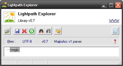
Naturally, one leaf and that’s all. Not really exciting. Let’s read the rest of the header up until File Table:
As mentioned in the pattern intro ANY matches any single byte except for EOF (which technically isn’t a «byte» anyway).
Surprisingly, this won’t work. We will read magic just like above but there won’t be anything else. As I have subtly introduced context prefix symbols last time (those 1, ?, ^ and others) I haven’t mentioned one important thing:
In Lightpath, context operates in two models: one-shot and loop. One-shot context, when entered, tries to match any of its children against the input and reports error upon failure. Looping contexts try to match their children infinitely – unless they have matched an END-context.
This switch occurs automatically. By default all contexts are one-shot unless they have an END-context or they have any of ordered or once-contexts (indicated with numeric or dot prefix – see last chapter).
So we have put 4 contexts into the root context (we don’t see it anywhere but all of model contexts without indentation belong to root). And this context is one-shot. Therefore, once any of its children matches it terminates. So magic has matched – and our processing has stopped. Without reaching other lines.
We can fix this in two equivalent ways:
There is a subtle difference between the two but we’ll leave it for advanced concepts. In many cases ordered and once-contexts are equivalent. Pick the one you like. My favourite is dot-notation as it doesn’t require changing other lines’ prefixes if I insert a new context in between.
Now if we load any of these models and ignore the warning we’ll see 3 more leafs created. Great! Now if you double-click on fileCount you will see that it starts at 00000010 and is 4 bytes long. Press on the  Preview button next to tart – hex dump window will open at this location:
00000008 63 56 31 2E 30 30 30 00 cV1.000.
-- HERE --
00000010 04 00 00 00 44 00 00 00 ....D...
These 04 00 00 00 bytes are our file count from the diagram in the beginning of this chapter. They say that this archive has 4 files. We’re yet to discover them but let’s trust the data.
We also have two other nodes from the Header:
- name offset – 44 00 00 00 at 00000014
- data offset – 6C 00 00 00 at 00000018
If you go to these offsets (44h and 6Ch) in your hex editor or in the same dump window you’ll see that they indeed mark the first file name’s symbol (s from sr006.mjo) and the first byte of first file’s data (M from MajiroObjX1.000).
So far so good. Time to go for File Table…
lp. "magic" % MajiroArcV1.000 \0 . "fileCount" % ANY ANY ANY ANY . "nameOffset" % ANY ANY ANY ANY . "dataOffset" % ANY ANY ANY ANY . "files" = "file" = . "hash" % ANY ANY ANY ANY . "offset" % ANY ANY ANY ANY
Oh, wait a second. It works but… we haven’t matched all the files. In fact, i see only the first one. Now for the most interesting part. How do we create loops?
The Looping Pattern
Life wouldn’t be so interesting if it would proceed from start to end in one monotonous streamline. Sometimes there are loops, sometimes there are choices. We have already dealt with choices in Lightpath – that’s just any context that doesn’t «loop». Now it’s time to tacke loops.
As mentioned above any context can be turned from one-shot to looping by placing an END-context or an ordered or once-context as one of its child. There might be many ENDs and many ordered and once-contexts, all mixed together in any order.
A looping context will end once an END-context that it contains has matched. This means that if there are 3 contexts like this outer won’t be terminated when END matches – only inner will be because it’s immediate parent of the END:
lp"outer" =
  "inner" =
    END
Lightpath automatically inserts an unconditional END for contexts containing ordered or once-children. This means that these two contexts:
lp"context1" =
  . "something" =
  END
"context2" =
  1 "something" =
  END
lp"context1" =
  . "something" =
"context2" =
  1 "something" =
So we can omit the END if it has a condition that always matches. This means that once all of our ordered/once contexts have executed parent context will automatically end. Quite convenient.
Let’s recall that File Table in MajiroArc contains 2 entries: hash and offset. Both are 4 bytes long and there are as many entries as there are files according to file count.
If we’d have be using C++ we’d write this:
for (int i = 0; i < file_count; i++) {
  uint hash = fread(f, 4);
  uint offset = fread(f, 4);
}
How do we pull this in Lightpath?
lp"files" =
  "file"? iteration fileCount$start toint <
    . "hash" % ANY ANY ANY ANY
    . "offset" % ANY ANY ANY ANY
  END
We’ve put END to make this context’s parent, files, switch to loop mode. END has no condition and will always match as soon as no previous contexts have matched. In our case – as soon as the condition of file has failed.
Here we are using expression (preceded by question mark, ?) – special commands that evaluate to either true or false value. If it’s true this node will «match», if false – next node will be tested. This is just like using =, % and other operators we’ve seen, only that the condition is more complex.
Lightpath expressions use Reverse-Polish Notation instead of our traditional notation with braces. In this notation operands (numbers, strings and so on) are pushed into the stack from left-to-right and operators (+ - < and so on) take these operands from the stack, placing back their result.
iteration fileCount$start toint <
…contains 4 items, evaluated from left to right:
- iteration – this is a function that returns how many nodes have matched inside current context.
- fileCount$start – this is a node reference. We are reading the value of node fileCount, in particular its start property.
- toint – this function converts Little-Endian integer into machine format.
- < – as you’d guess it’s our «less-than» operator.
The Iteration Spinner
First of all let’s see what iteration is. Suppose we have this model:
This simple model will match strings like out.in.foo.bar. following each other in succession. Like this one:
out.in.foo.bar.in.foo.bar.out.in.foo.bar.in.foo.bar.in.foo.bar.Once applied you will get this tree (we’re starting to go deeper – 3 levels now, be proud!):
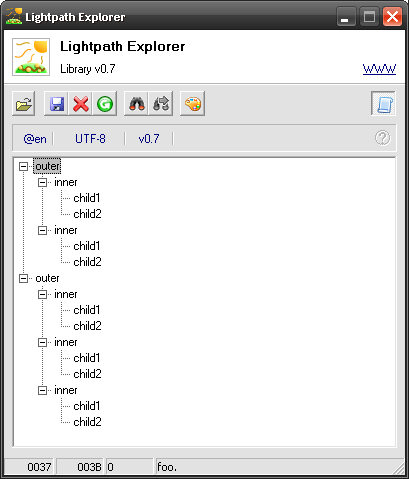
If you think of Lightpath contexts as a series of nested fot loops (which deep inside it essentially is) then iteration is simply the value of that int i variable.
for (int rootIteration = 0; rootIteration <= 2; rootIteration++)
  /* Now iwthin the root context with nodes outer, outer */

  for (int outerIteration = 0; outerIteration <= 1; outerIteration++)
    /* Now iwthin first outer\ context with nodes inner, inner */

    for (int innerIteration = 0; innerIteration <= 1; innerIteration++)
      /* Now iwthin first outer\inner context with nodes child1, child2 */
In other words: once a context is entered its iteration counter is zero (0). Once the first child node matches iteration counter becomes one (1). Once another node matches it becomes two (2) and so on – until the context is quit.
Nested contexts get their own independent iteration counters.
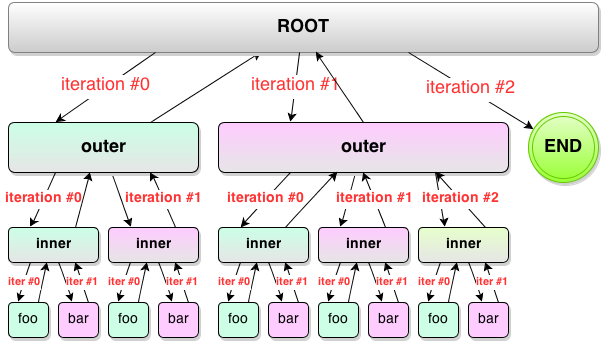
- Contexts which execute during 1st iteration (that is, 0)
- Contexts which execute during 2st iteration (1)
- Contexts which execute during 3rd iteration (2) – note that END is a regular context and it’s executed during iteration #2 as well
Node References
Iterations sorted out we have one more concept to grasp: a node reference. Remember those URLs and Windows/Linux paths you always copy/paste? Node references are basically the same: it’s a path of nodes, each component separated by forward (\) or backslash (/). These two are interchangible. By convention Lightpath uses forward slashes (node\child).
This path can also be prefixed with either of these symbols:
- One or more dots as in ..parent's_parent – one dot goes one level up, two dots – two levels up and so on until root is reached. This is the same as writing ..\..\ in Windows (../../ in *nix).
- One or more slashes (either \ or /) as in \\root's_child. These are the opposite of dots – they go one level down from the root until current node is reached. So if current node is root\parent\child\current then path \\child_of_parent will refer to node named child_of_parent belonging to node root\parent. If we have path \root_child then we are referring to child root_child of the root node.
Quite often you don’t want a node per se but its property. For example, if you want to access the number of files that you have read in your model earlier (just like in our case!). For this use regular node path as described above but add $propertyName to the end. If you include just dollar symbol ($) but omit property name itself inner will be implied.
- parent\child\node
- node of child of $$parent%% relative to current node.
- parent/child/node
- The same as above but using *nix notation (don’t mix both kind of slashes in one path).
- \\\child\three\levels\down
- Goes 3 levels down from the root node and finds node named child, of which it finds three, of which levels and, finally, down.
- ...node\three\levels\up
- = Just like above but goes from current node up so it looks up the parent, that parent’s parent and that parent’s parent to find node, of which it searches three, of which – levels and, finally, node named up.
- child$prop
- Searches for current node’s child named child and retrieves that node’s property named prop.
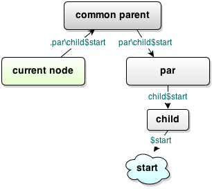
- .par\child$start
- Takes current node’s parent, finds node named par, then looks for child among parent’s children and returns property named start (of child).
- $inner
- Empty path always refers to current node. So we’re reading property inner of the current node.
- $
- If we omit property name inner is implied; if we omit node path – current node is implied. Therefore, we are reading property inner of the current node.
- .child$
- Reading property inner of the parent’s node named child.
Getting Back Up
Finally we can get back to our expression and explain what it does:
iteration fileCount$start toint <
First, we call function iteration which returns the iteration number of the current context. So if we have this:
lp"files" =
  "file"? iteration
    ...
Then ? iteration part will return 0, 1, 2 and so on – once per each matched file.
After iteration returns the number it’s placed on stack. «Stack» is like a stack of paper – at first you have an empty desk, then you put a paper on top of it, then another paper comes in and you place that on top of the first – and so on until you’ve covered all the light from the window.
If at some point to decide to bring that pile down you will start from the paper on top – that is, which you have last placed there. Then you will take off less recent paper – you’ve placed it before the one you’ve just dealt with. And so until the bottom where you’ll take the first piece of paper, that has been waiting for all others, and say: «Now I know why it stucks!»
So, we have one element on our stack and it’s iteration number. Then we read property start of node fileCount. Why start? Let’s remember out model:
lp"fileCount" % ANY ANY ANY ANY
start refers to the part of stream matched by condition. Here it’s 4 bytes, ANY ANY ANY ANY. inner property refers to part of stream matched by all child context of this context (it doesn’t include start). If context has no nodes then inner is always empty. For looping contexts there’s also end property that contains portion of data matched by END node that has terminated this context.
So we’ve read the file count and placed it on top of iteration index. However, «file count» now is just a series of 4 bytes: 04 00 00 00. It’s not a number, it’s a string – a number can be 1, 2, 4, 8 bytes long, be signed or unsigned, be fractinal and can even be written using different endianess. So to make this string «real number» to which we can apply math we call toint. This function takes one operand – a string – off the stack and treats it as having Little-Endian byte order and being 1, 2, 4 or 8 bytes long (it errors otherwise) to convert it into 8, 16, 32 or 64-bit integer correspondingly. The result is placed back on stack, effectively replacing the operand (in our case file count string is replaced by file count number).
Now we have the last < operator. It takes off one operand, then another (our stack becomes empty) and compares them. If iteration < fileCount$start then we get value true and our condition matches (file node is created, its children begin executing and so on). If they don’t match we get false and processing might stop if this context an ordered or once – just like with other conditions like = foo and % BAR.
A more complex example. We have this RPN expression:
a b 1 + <
Let’s see how stack is filled up:
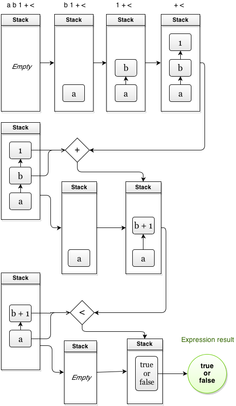
As you see this is equivalent to the following expression in the notation more familiar to us:
a < (b + 1)
This fancy syntax requires a bit of a practice but it’s more than doable. In fact, advanced scholars use RPN over traditional notation because, according to them, it gives less chance for errors and is faster to calculate. Welcome to the circle of science!
Reading File Table
This was some pile of new info but I’m sure you’ve climbed on top before hearing worried voices. So let’s continue before they sound in panic.
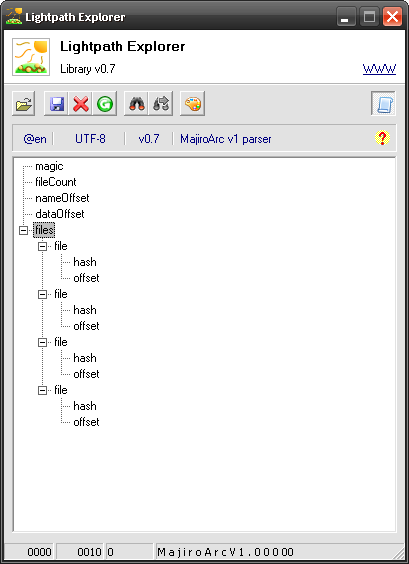
Cannot find node 'fileCount' relative to '\files' referenced
in RPN expression (n = 0) 'iteration fileCount$start toint <'.
But of course! We’re typing to access \fileCount node file being inside \files. This means that we are trying to read \files\filesCount. Let’s correct it by adding leading slash or dot so it becomes \fileCount$start. Hurray!
Inheritance Chain
Any review of Lightpath isn’t complete without at least scratching on its inheritance machanism. This is a very powerful system which idea is similar to class inheritance in programming languages but is pushed to the limits.
In languages where multiple inheritance isn’t possible you write something like this (Delphi code):
pascalTMyBaseClass = class
  SomeNum: Integer;
end;

TMyChildClass = class (TMyBaseClass)
  NewNum: Integer;
end;
Here, TMyChildClass gets all the members of TMyBaseClass. So it has two fields – SomeNum and NewNum.
Languages with multiple inheritance like C++ and Ruby (with its mixins) allow you to add more classes into the common bowl so first you merge fields of base class one, then base class two and so on. If field names collide at some point the latter overrides the one defined earlier in the chain.
Lightpath allows for similar inheritance mechanism too, in its own form:
lp(dword)
  "dword" % ANY ANY ANY ANY
dword "fileCount"
dword "nameOffset"
«dword» is a common term which stands for «double word» – 32-bit unsigned integer on Windows although technically a «word» means value native to your CPU which today in most cases is 64-bit. Thus «double word» would mean a 128-bit value.
Something new we see here. The first line defines so-called off-context «context». Such contexts are not tested against input. They are inexistent; even when their parent context tests each of its children against the data off-contexts are never tested.
However, they play important role: they define «templates» (or «classes» in OOP terms) that can be inherited by other nodes – both in-context and off-context. When a node has a name and that name matches any of the off-context node nearby – the first node gets everything the off-context node contains. This way our example is identical to the following model, except it’s shorter:
lp"fileCount"
  "dword" % ANY ANY ANY ANY
"nameOffset"
  "dword" % ANY ANY ANY ANY
Contexts inherit not just children but also conditions. In our example fileCount and nameCount have no conditions assigned, not even an = in the end. This model is again equivalent to the two above but is even shorter:
lp(dword) % ANY ANY ANY ANY
dword "fileCount"
dword "nameOffset"
There’s a potential pitfall. A context will only be marked as inheriting when it has no condition assigned, as in our example, or if its name starts with @ symbol. So, returning to our first sample:
lp(dword)
  "dword" % ANY ANY ANY ANY
@dword "fileCount" x FF FF FF FF
dword "nameOffset"
lp"fileCount" x FF FF FF FF
  "dword" % ANY ANY ANY ANY
"nameOffset"
  "dword" % ANY ANY ANY ANY
However, should we omit the at symbol then we’ll get this:
lp"fileCount" x FF FF FF FF
"nameOffset"
  "dword" % ANY ANY ANY ANY
As you see fileCount didn’t inherit anything from dword. We could’ve omitted dword before "fileCount" too with the same effect.
Another pitfall is this: if you don’t include any condition context will be assumed to be inheriting and the best thing that will happen is Lightpath telling you it can’t find base context (it will refuse to load such a model). Worse would be that it could find it and added child nodes you didn’t account for.
Because of this always include an empty condition like this to ensure you are not mistakingly inheriting a context:
empty "condition" =
Inheritance isn’t limited to only one level. If you have a complex model then you can inherit contexts from any other off-context defined above or on the same level where the inheriting context is.
To illustrate this point (blank lines are ignored inside a model):
Hey, doesn’t it look better with all the ANY ANY ANY ANY stuff gone? I bet it is. And it even reads more naturally: «a double word “fileCount”.». Sounds good.
Let’s go ahead. We have File Table covered – with all the hashes and offsets. Next is the File Names list. As you remember it’s a series of Shift-JIS strings, each terminated by a zero byte. Let’s also not forget that we have an End-of-File entry and put it before our list of names.
You must’ve got the clitch on Lightpath by now so this should be self-explanatory. We’re reading each name context for as many times as there are files according to fileCount. This context has two nodes and is in looping mode: first node matches all symbols except for zero byte (syntax here resembles regular expression notation) and second matches only zero byte. Naturally, a string contains non-zero bytes and is terminated with one. So we write.
And it actually works. Before long we’ve got the list of file names on our place. Perfect job!
At this point we could’ve called this a day – after all, we got offsets and names, archive’s parsed, right?
Well, if you’re not up to a high then it might be said so. But what if we move names under each file entry? What if we read data too and turn this model into the real file tree – and actually extract the data? Can we do that?
Sure. No problem. Carry on while the sun’s high.
The Node Formula
Today’s lessor is rich in concepts and so I’ll throw another one onto you. It turns out that my earlier description of node references – or just paths – was incomplete. Apart from nodes and properties we can also put expressions there. For short we’ll call them formulae for this is what they are.
Let’s see what our problem is:
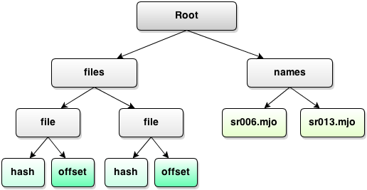
It’d be best to get rid of the separate names branch and move everything under corresponding file branches:
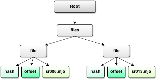
That’s something we can do using by picking the right formula. Now we have:
lp. "names" =
  "name"? iteration \fileCount$start toint <
    ; Contents...
lp. "names" =
  "\+files\file[n]\name"? iteration \fileCount$start toint <
    ; Contents...
I haven’t said it before but in context "path" you don’t have to put just letters to create a node right under the parent of this context. You can specify a full node reference – and it can be well ouside the parent and can create or append contents to new or existing nodes in the produced tree. That’s what we’ve done above:
- +files
- This part refers to node files present under root (because it starts with a slash). Plus sign (+) means that we don’t want to create a new node, we want to append contents to existing node. Since we have to create at least one new node we can’t use plus sign with the last path component. But here it’s the first component so everything’s okay.
- file[n]
- This is the main kicker. Just as programming languages use square brackets to refer to elements in an array Lightpath uses them too – except that here you can put any math expression like n*5/2-1+n – and it will evaluate to some number. This number is used to find a child by index within the parent (in our case we are searching amoung children of \files0. Indexes start from zero, just like iteration counter. If there’s no child with that index new child is created (but it won’t necessary have the given index). That said, n is that iteration counter as described earlier.
- name
- This part is simple. New node named name is created under file child with index n.
Now, if we are reading the first file name in the list we’ll get this path:
\files\file[0]\name
And it refers to the first files\file node under which we place node name, filled with first file name. Exactly what we need. Same goes for the rest of files. Now if you put this model into Lexplore you will see that we indeed have got a good result – all names put under corresponding file entries. Which means we can remove the "names" node altogether.
Data in My Pocket
Now we’ll go for the last part of the puzzle: reading the data. Once done, we’ll have a near tree like this:
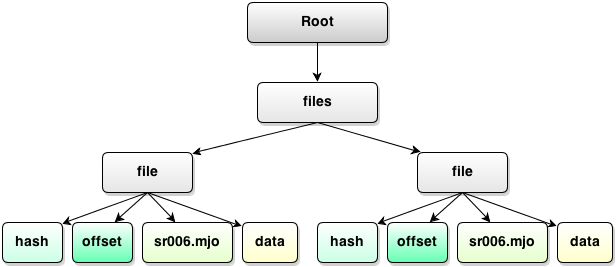
This is, in fact, a complete tree form of the archive, fully ready for convenient processing because we have laid out all the structures and effectively «unflattened» the data and given it a real gas state.
We’ll be creating data nodes just like names – using formulae. However, we’ll need a special expression because unlike with names we don’t know the length of data – we only know its offsets.
lp.
  END? iteration \fileCount$start toint =
  "\+files\file[n]\data"? \files\file[n+1]\offset$start toint skipto
This will do the job. First line (the dot) simply defines a new context with no condition (i.e. it always matches). Inside there’s an END node that will be matched once iteration is equal to file count – and once it is parent context will be termianted and no more data will be read.
The second child is interesting. First we see the familiar reference to the file node where we are putting new node data. Then we see that a similar reference appears in the expression. Let’s break it down:
- files\file[n+1]\offset$start
- We access property start of node offset located under file which is children number n+1 of its parent node, files (located in the root). n+1 means that that node is next to current node. In other words if we are reding data of the first file (iteration 0) then we’re accessing offset of the next file – because, of course, first file ends when the second file starts.
- toint
- A familiar function that converts Little-Endian string-number into a proper integer. So we got an offset on stack.
- skipto
- This function positions input stream on the given offset. It doesn’t go backwards (if offset you’re trying to position on is prior to current input position nothing happens).
So it goes like this: enter first file’s data loop, skip to the next file’s data offset, then enter second file’s data loop, skip to the third file and so on until END matches which happens exactly when iteration counter becomes equal to fileCount and given that file count is 1-based while iteration index is 0-based this END matches when we’ve read all files and are about to start reading next file that isn’t present.
Try to apply this new model to our scenario.arc. Oh, we get an error. Let’s see…
Cannot find node '\files\file[n+1]\offset' relative to '\' referenced
in RPN expression (n = 3) '\files\file[n+1]\offset$start toint skipto'.
But of course. We have 4 files in our archive (\fileCount = 4). The error says that n is 3. Thus we are reading the last, 4th, file (since n is 0-based) and the engine cannot find node file which has index 4 (because it’s n+1). Index 4 means it’s the 5th file entry. But we only have 4 entries: one per each file.
Lucky for us Majiro authors have put an End-of-File entry just in this case. Let’s refactor our model a bit and move endOfFile contaxt under files, thus adding extra file entry which will be used when we read file data.
You could move that entry under . "files" = for the same effect.
If you now open Node Properties of any data node you will see proper Start position and length. If you click on the Save  button Explore will dump the data from that offset to that length effectively extracting data from the archive. And the best thing, of course, is that it’s not limited to MajiroArc – it will work the same way for any data we have provided a model for.
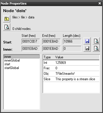
Now our MajiroArc model is truly complete. It took us some sweat but we’re now Binary Kings. Kudos! Next chapter will be a breeze and will show us a few more great ways to make our reverse data engineering go smooth.
Question Marks
Congratulations on covering the basics and more advance aspects of Lightpath. To hone your new skills let me offer a small task: describing ZIP file format. It is tangled and I don’t ask for the complete support but we can easily do the basics. Here’s the original specification – scroll down to 4.3.7 Local file header and you will see a concise list of fields along with their sizes. After these fields compressed file data follows.
Here’s what I’ve got after applying my model to the sample archive:
